Training Autoencoders on ImageNet Using Torch 7

If you are just looking for code for a convolutional autoencoder in Torch, look at this git. There are only a few dependencies, and they have been listed in requirements.sh

Introduction

I have recently been working on a project for unsupervised feature extraction from natural images, such as Figure 1.

I will save the motivation for a future post. One of the methods that I was exploring at the time was autoencoders. Since most of the code in our office is written in Lua, using Torch was the logical choice. At the time, I was still learning how to create a working network architecture, so I did a lot of learning on relevant papers, such as AEVB and AlexNet. I was also looking into tutorials on how to actually write an autoencoder, for example the excellent blog post by Mike Swarbrick Jones.

To the best of my knowledge, there are no publicly available examples for writing autoencoders on color images. There are, however, several examples on how to write an autoencoder for the MNIST dataset. It might be easy for seasoned machine learning scientists to extend the architecture from grayscale to color images, but for me it was non-trivial. The goal of this post is to provide a minimal example on how to train autoencoders on color images using Torch.

The Big Picture

Figure 2. shows the major components of an autoencoder. The input in our case is a 2D image, denoted as \(\mathrm{I}\), which passes through an encoder block. The purpose of this block is to provide a latent representation of the input, denoted as \(\mathrm{C}\), which we will refer to as the code for the remainder of this post. This code is subsequently passed through a decoding block, denoted as \(\hat{\mathrm{I}}\), which generates an approximation of the input.

Figure 3. shows the components of the encoder that is used throughout this post. Most of the computation is performed using the three convolution layers, i.e. \(Conv_{1..3}\). Without non-linear elements, encoding would be a linear dimensionality reduction similar to principal component analysis (PCA), since convolution is a linear operator. Since the space of images is not guaranteed to lay on a hyperplane, it is customary to add a non-linear element to the output of convolution layers, which in this example is a rectifier linear unit (\(ReLU\)).

The encoder also has two max-pooling elements after the second and third convolution layers. Max-pooling can be thought of as a grid that summarizes activated neurons from the previous layer. It has been suggested that networks that do include pooling layers are less likely to overfit.

The final layer of the encoder is a fully connected layer, which serves to aggregate the information from all the neurons in the previous layer. This layer is essentially a linear mapping of its input. The code is simply the output of this layer.

The decoder component of the autoencoder is shown in Figure 4, which is essentially mirrors the encoder in an expanding fashion. The output of the decoder is an approximation of the input.

Autoencoder Class

We will first start by implementing a class to hold the network, which we will call autoencoder. Lua does not have a built in mechanism for classes, but it is possible to emulate the mechanism using prototypes. We will define the autoencoder class and its constructor in the following manner:

autoencoder = {}
autoencoder.__index = autoencoder

setmetatable(autoencoder, {
  __call = function (cls, ...)
    return cls.new(...)
  end,
})

function autoencoder.new()
  local self = setmetatable({}, autoencoder)
  return self
end

Next, we will define a initialize() method. This method sets up the autoencoder with de/convolution, ReLU, un/pooling and linear blocks as described in the previous section. The initialize() method has the following structure:

function autoencoder:initialize()
  self.net = nn.Sequential()
  # network layers are defined here:
  # layer 1
  # layer 2 ...
  # layer N
  self.net = self.net:cuda()
end

nn.Sequential() defines a container for the network that behaves in a serial manner, i.e. the output of one block is the input to another. The layers are defined in the commented code block above, i.e. layers 1-N. The last line, i.e. self.net:cuda() copies the network to the GPU for faster training.

Now that we have the structure in place, we can start adding layers. We assume that the input to our network are 64\(\times\)64 RGB images. For this post, we will hard-code layer sizes, but it is possible to for layers to infer their size based on input and model parameters. For non-convoutional layers, computing sizes is trivial. For convolution layers, the relationship between the dimensionality of inputs and outputs is the following:

output = (input - kernel_size) / stride + 1

The first layer is convolutional. We will add it to the network using the following code snippet:

self.net:add(nn.SpatialConvolution(3, 12, 3, 3, 1, 1, 0, 0))

This defines a convolution layer that has 3 input channels, 12 output channels, a 3\(\times\)3 kernel and a stride of 1. We will follow this layer with a ReLU element, which is simply a non-linear activation function:

self.net:add(nn.ReLU())

Fully connected layers are defined in the following manner:

self.net:add(nn.Linear(24 * 14 * 14, 1568))

Similarly, we can add a pooling layer that downsamples with a factor of 2\(\times\):

local pool_layer1 = nn.SpatialMaxPooling(2, 2, 2, 2)
self.net:add(pool_layer1)

Unpooling layers require the pooling mask. So, we can define them using this code snippet:

self.net:add(nn.SpatialMaxUnpooling(pool_layer1))

Finally, we are going to Connect all the layers in the initialize() method. This is shown in the following code snippet:

function autoencoder:initialize()
  local pool_layer1 = nn.SpatialMaxPooling(2, 2, 2, 2)
  local pool_layer2 = nn.SpatialMaxPooling(2, 2, 2, 2)

  self.net = nn.Sequential()
  self.net:add(nn.SpatialConvolution(3, 12, 3, 3, 1, 1, 0, 0))
  self.net:add(nn.ReLU())
  self.net:add(nn.SpatialConvolution(12, 12, 3, 3, 1, 1, 0, 0))
  self.net:add(nn.ReLU())
  self.net:add(pool_layer1)
  self.net:add(nn.SpatialConvolution(12, 24, 3, 3, 1, 1, 0, 0))
  self.net:add(nn.ReLU())
  self.net:add(pool_layer2)
  self.net:add(nn.Reshape(24 * 14 * 14))
  self.net:add(nn.Linear(24 * 14 * 14, 1568))
  self.net:add(nn.Linear(1568, 24 * 14 * 14))
  self.net:add(nn.Reshape(24, 14, 14))
  self.net:add(nn.SpatialConvolution(24, 12, 3, 3, 1, 1, 0, 0))
  self.net:add(nn.ReLU())
  self.net:add(nn.SpatialMaxUnpooling(pool_layer2))
  self.net:add(nn.SpatialConvolution(12, 12, 3, 3, 1, 1, 0, 0))
  self.net:add(nn.ReLU())
  self.net:add(nn.SpatialMaxUnpooling(pool_layer1))
  self.net:add(nn.SpatialConvolution(12, 3, 3, 3, 1, 1, 0, 0))

  self.net = self.net:cuda()
end

Data Preparation and IO

For me, I find it easiest to store training data is in a large LMDB file. Caffe provides an excellent guide on how to preprocess images into LMDB files. I followed the exact same set of instructions to create the training and validation LMDB files, however, because our autoencoder takes 64\(\times\)64 images as input, I set the resize height and width to 64.

Reading data for either training is done through a lmdb_reader class which takes a path to a LMDB folder as input for its constructor. For now, ignore the details of this class. What is important is that data is read in batches and returned as {input, target=input} pairs.

In the future, I might write a post on how to write the class. But for now, a seasoned developer can easily dissect the reader class and the accompanying protobuf file.

Training

Normally, neural networks are trained on large datasets that are orders of magnitude larger than the available CPU/GPU memory. As a result, the network is presented with batches of data during the training in the hopes that by each incremental observation of the input, the distribution of inner layer weights can be accurately approximated. One of the most popular methods for optimizing the value of inner layer weights is the stochastic gradient descent SGDC.

The training script is provided under /scripts/train.lua. To run it in the root folder with default parameters, simply call:

th scripts/train.lua /path/to/imagenet_train_lmdb/

Training our autoencoder is simple using SGDC. First, we need to create an instance of our autoencoder and initialize it:

ae = autoencoder()
ae:initialize()

Since our data is continuous, we will use the mean-squared error as the loss function for training. We can now set up SGDC optimizer for training. This can easily be done using the following snippet:

criterion = nn.MSECriterion():cuda()
trainer = nn.StochasticGradient(ae.net, criterion)

To start training, we simply read a data batch and call the :train() function on the batch:

for t=1, options.epochs do
  print('Epoch ' .. t)
  data_set = imagenet_reader:get_training_data(options.batch_size)

  trainer:train(data_set)

end

Testing and Results

Once the training is finished, we can pass images from the validation set through the autoencoder in forward mode. If the output matches the input, the autoencoder has been successfully trained. The testing script is provided under scripts/test.lua. To run it in the root folder with default parameters simply call:

th scripts/test.lua ./path/to/trained/network.bin /path/to/imagenet_val_lmdb/

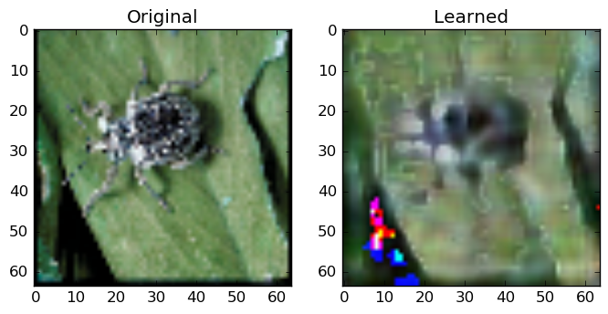
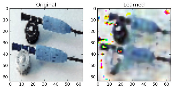
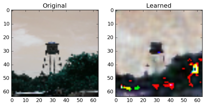
Below are some of my results:

As you see, the network can approximate the general properties of its inputs. In Figure 5., the learned representation is blurry compared to the original, however, the network managed to capture the general color of the brown beetle and the surrounding green leafs. In Figure 6., the fishing equipment can be distinguished in the learned representation, however, the network has failed to correctly recover some pixels. These pixels have distorted color values. The same shortcomings are also present in Figure 7.